Past a certain load, one machine runs out — and a bigger GPU is not the answer, since the biggest is already in the node. The fix is a fleet: many replicas serving one model.
It is a distributed system like any other, only with unusually expensive, unusually stateful workers. NVIDIA Dynamo is one open-source framework for running that fleet, and what makes it worth studying is the design more than the code: its architecture doc is the clearest overview of the whole problem I have found. So these are my notes on how a fleet holds together, organized around the way Dynamo structures and manages one.
From one replica to many
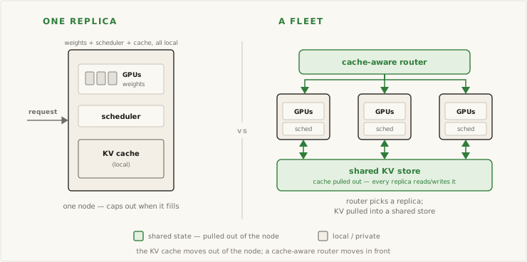
One replica is a single model instance: the weights loaded across some GPUs, a scheduler, and the key/value (KV) cache for the requests it is serving. The continuous-batching loop lives entirely here — re-form the batch every iteration, page the KV cache in fixed blocks, keep the GPU busy. It scales until the machine is full, and no further.
Past a full machine, you add replicas behind a load balancer, the way you’d scale a stateless web service. Except inference replicas aren’t stateless. A replica that just processed a long prompt is holding that prompt’s KV cache; the next turn of the same conversation wants that cache, and only that replica has it. Round-robin throws it away.
So the load balancer in front has to be cache-aware, and the state behind the replicas has to be locatable and movable — a router and a shared index a single server never needed. Dynamo names these directly: a KV-aware router in front, and a KV cache the fleet can locate and move behind — tracked by a shared prefix index, not pooled in one central store. Almost everything else is a consequence of those two.
Memory, compute, network
A node hits one of three limits. They are worth naming up front because they are independent — you can be nowhere near the compute limit and still be blocked by the memory one.
Memory. The weights and the KV cache share the same high-bandwidth memory (HBM), and both are large. A 70-billion-parameter model in 16-bit precision is about 140 GB of weights — already past a single 80 GB accelerator. Llama 3.1 405B is roughly 810 GB in fp16; DeepSeek-V3, trained in FP8, is about 671 GB. Those do not fit on one node. And the KV cache grows on top of the weights, with concurrency and context: for a 70B model with grouped-query attention (GQA), one token of context is about 0.32 MB of cache across all layers, so a single 128k-token request is roughly 40 GB — for one user. (These are rough sizings from the published configs, not measured footprints; real deployments add activations and framework overhead.) Serve many users at long context and the cache, not the weights, exhausts memory.
Compute. Prefill — reading the prompt — is compute-bound: it processes every prompt token in parallel and saturates the GPU’s math units. Decode is the opposite, memory-bandwidth-bound, one token per step. On a single node the two compete for the GPU: a large prefill stalls the decodes sharing the machine, and no batching split satisfies both at once. (Sarathi-Serve reports naive hybrid batching inflating time-between-tokens by up to 28×, author-reported.) Sustaining prefill throughput under real load means spreading it across more GPUs than one node holds.
Network. The moment a model is sharded across GPUs, they have to talk every forward pass. Tensor parallelism does an all-reduce at each layer; a mixture-of-experts (MoE) model adds an all-to-all to route tokens to experts. Both sit on the critical path — one vendor’s measurements put the tensor-parallel all-reduce at up to about 30% of end-to-end latency in specific configurations, and MoE’s all-to-all in a similar range. Disaggregating prefill from decode adds one more transfer: the KV cache itself, handed from the machine that built it to the machine that generates from it. Communication is a first-class cost here.
Dynamo’s structure is a set of answers to these three limits — tier the cache so it outlives GPU memory, split the phases so neither starves the other, and move state fast enough that the transfer is cheap. The rest of this is those answers.
The three planes
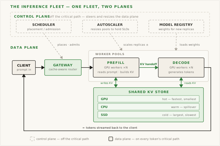
Dynamo’s design doc splits the system into three planes — a request plane, a control plane, and a storage & events plane — described as three cooperating concerns: a fast request path, a responsive control path, and a resilient state path. Which plane a part lives in predicts how it scales and how it fails, so it is the first distinction to apply.
The request plane is every token’s critical path — Frontend → KV router → prefill worker → KV transfer → decode worker → tokens streamed back — and its latency is what the user feels. Three parts sit on it:
- The Frontend. An OpenAI-compatible HTTP server that terminates and normalizes the request, sitting on Dynamo’s Rust DistributedRuntime.
- The KV router. It picks a worker by load and KV-cache overlap — routing the request to the worker that already holds the relevant prefix rather than round-robin. Dynamo is engine-agnostic: the workers themselves run vLLM, SGLang, or TensorRT-LLM.
- The prefill and decode workers. Two pools — one that reads prompts and builds KV cache, one that generates tokens from it. Whether they are actually two pools or one is the design choice a later section is about.
The storage & events plane is the KV state and its movement. It is the plane a two-plane data/control split omits, and the one Dynamo separates deliberately:
- KVBM — the KV Block Manager — treats KV as a tiered resource, offloading blocks across GPU → CPU → SSD → remote storage so effective context outlives GPU memory.
- NIXL — the NVIDIA Inference Xfer Library — is the point-to-point engine that moves blocks between workers and memory tiers, over NVLink, InfiniBand, or whatever interconnect is fastest.
- KV events are how the plane reports its state: each worker emits an event when it caches a block and when it evicts one, and those events are how the router learns which worker holds which prefix.
Pulling this out is the structural move. A cache hit turns a prefill into a lookup, so the KV state is on the critical path; yet the router steers on its events and the autoscaler watches its utilization, so it also answers to the control plane. Giving it its own plane is what turns the KV cache from an incidental part of the data path into a storage system with its own tiers, eviction, and failure modes.
The control plane manages the other two without being on their path, on a slower clock — seconds and minutes, not milliseconds:
- The Planner is the autoscaler; it has its own section below.
- The Dynamo Operator reconciles the deployment to its desired state on Kubernetes — health, placement, replica counts.
- ModelExpress loads and streams model weights to new workers, which is the difference between a new replica coming online quickly and one that stalls behind a slow, serial pull of its weights.
When the control plane is down, the request plane keeps serving on its last decisions — no new scaling, stale routing — which the fleet can tolerate for a time.
One request ties the three together. The client hits the Frontend; the router picks a prefill worker, which computes the prompt’s KV and hands back transfer metadata; the router picks a decode worker, which pulls that KV over NIXL and starts generating; tokens stream back through the Frontend; and as blocks are cached and evicted, KV events update what the router knows for the next request. Request plane for the path, storage & events for the state, control plane monitoring both.
Three Control Loops
Over those planes Dynamo names three Control Loops — Serving, Planning, and Resilience. Only one of them literally ticks on a timer; the other two are names for a job the fleet is always doing, and naming them ensures each of these jobs has a clear owner.
The Serving Loop keeps request-plane latency low across Frontend, router, prefill, and decode. This is the steady state — the single replica’s continuous-batching loop, now spread across the fleet.
The Planning Loop is the one that ticks, and it is where fleet management actually happens. The Planner is an autoscaler driven by service-level agreements (SLAs): it profiles the workload and right-sizes the prefill and decode pools to hold its latency targets at the lowest cost. It sizes the two pools independently, because prefill is compute-bound and scales with input length while decode is memory-bound and scales with concurrent sequences and KV usage — one replica count can’t capture both. It scales on inference-aware signals — KV-cache utilization, queue depth, per-iteration timing — not CPU load, and it targets Time-To-First-Token and Inter-Token Latency directly (the SLA defaults are 500 ms and 50 ms). On Kubernetes it applies a decision by editing the deployment’s desired prefill and decode counts, which the operator reconciles into workers. One open edge: Dynamo’s docs don’t specify whether a scaled-down worker is drained of in-flight work or killed mid-request — the planner-design page states only that it scales by ±1 per interval. The Resilience Loop’s graceful shutdown and request migration exist precisely because autoscaling a stateful fleet is not the same as autoscaling web pods.
The Resilience Loop keeps the fleet serving under failure: health checks to find dead workers, discovery liveness to drop stale endpoints, graceful shutdown to drain in-flight work, request migration and cancellation, and load shedding to keep an overload from cascading. Each of those is a hard problem in its own right; the loop is the name for the fact that something has to own them.
Scaling the control plane and router
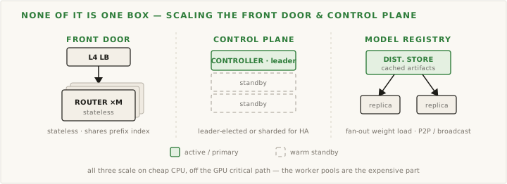
Figure 2 draws the router, the control plane, and the weight source as one box each. At fleet scale every one of them is a pool, because a control plane with a single point of failure takes the whole fleet down the moment it dies. These scale cheaply — on CPU, off the GPU critical path.
- The router is a set of replicas behind an ordinary L4 load balancer. Routing is close to stateless, with one catch: the cache-aware decision has to know which worker holds which prefix, so the routers share that prefix index — built from the storage & events plane’s KV events — rather than each one guessing alone.
- The control plane runs replicated for availability. On Kubernetes the Dynamo Operator is a controller, and controllers get availability the standard way — leader election, one active instance with warm standbys behind it — which the platform gives you largely for free.
- Weight loading is not one file server but a fan-out path. ModelExpress loads a model once and streams the weights to new workers GPU-to-GPU, because standing up a replica means moving hundreds of gigabytes now, and pulling that serially from one origin is how a traffic spike becomes an outage. NVIDIA presents it as a way to shorten replica cold start.
The worker pools are the expensive, GPU-bound part the Planner sizes. Everything else here is cheap enough that it is easy to forget it has to scale at all.
Aggregated, disaggregated, or hybrid
Set the control plane aside: the worker pools carry the one design decision that shapes everything else — do prefill and decode run on the same workers, or different ones? Dynamo is built to run them disaggregated — its request narrative, its NIXL transfer, and its per-pool Planner all assume the split — but the split is a configuration, not a requirement.
Aggregated replicas — one colocated pool, what Dynamo calls an aggregated deployment — do both. Every worker prefills and decodes, batching the two phases together, the classic vLLM continuous-batching design. It is simple, and it is where most deployments start. Its problem is the compute limit from earlier: the two phases interfere, and one replica’s parallelism and memory plan has to compromise for both.
Disaggregated serving splits them into separate pools — a prefill fleet and a decode fleet, each with its own hardware, parallelism, and scaling. DistServe and Splitwise made the case that this raises goodput and lowers cost per token by removing the interference (Splitwise reports 1.4× throughput at 20% lower cost in one configuration, author-reported; DistServe reports up to 7.4× at tighter latency targets, OSDI’24). The cost of it is the KV transfer — the cache has to cross the network from prefill to decode — which is exactly what NIXL exists to make cheap. Dynamo runs this as a reconfigurable x prefill workers to y decode workers, and lets you change the ratio at runtime as the traffic mix shifts.
Hybrid is where much of the field sits. You can attack the prefill/decode interference without physically separating the pools: Sarathi-Serve’s chunked prefill slices a big prefill into the decode stream so neither starves, keeping colocated replicas but bounding the latency. And a real fleet might disaggregate long-context traffic while colocating short requests. It is a workload decision, not a default.
What to measure
A fleet is judged on goodput: the request rate it can serve while still meeting its latency targets. The distinction from raw throughput is what matters — you can inflate tokens-per-second by batching so aggressively that half the requests miss their deadlines, and those tokens are served but useless. DistServe popularized the term for LLM serving precisely to stop that inflation. Dynamo’s Planner is stated in TTFT and ITL SLA terms rather than in goodput, but holding those at the lowest cost comes to the same thing.
The latency targets are two, one per phase:
- Time-To-First-Token (TTFT) — submission to the first token. Dominated by prefill, so it grows with prompt length. This is responsiveness.
- Time between tokens (TBT) — which Dynamo calls Inter-Token Latency (ITL) — the gap between streamed tokens after the first. Dominated by decode. This is smoothness, and it is measured inconsistently: a per-token interval you can take a p99 of, or an average that hides stalls.
Targets are stated at the tail — “99% of requests under X ms TTFT and Y ms ITL” — and SLO attainment, the fraction of requests that clear both bars, is what goodput is measured against (SLO: service-level objective). Underneath, the number the business watches is cost per million tokens, which is just the fleet’s hourly bill divided by the tokens it serves within SLO. Every architectural choice is ultimately an argument about one of these numbers — and they are exactly the numbers the Planner’s targets are stated in.
The shape, and the open problems
Put it together. Requests arrive at a Frontend and KV router, which place them on a prefill pool and a decode pool that each keep a tiered KV cache — KVBM — moved between them by NIXL, with KV events feeding the routing; a Planner sizes the two pools to hold its latency SLOs at the lowest cost; the operator keeps the whole shape reconciled; and ModelExpress keeps weights ready to stand up new workers. Three planes, three control loops, three limits, one metric.
Each part is a problem of its own: disaggregation and what the KV transfer costs; routing, and why round-robin is the wrong default; the distributed KV cache as a storage system with its own tiers and eviction; and the parallelism that serving uses, which is not the parallelism training used. Then the Resilience Loop’s own work — the three things an overview like this leaves out: what happens when traffic spikes faster than the Planner can react, what breaks when a GPU dies mid-decode, and how a fleet recovers state that was only ever held in memory.
That is the shape of it. More notes as I go.