Attention, from First Principles

Attention lets every token look back over the sequence and pull in the context it needs — and it’s exactly where the KV cache comes from. In this post, we will explore what attention is and how it is constructed.

What attention replaced

Until 2017, sequences were modeled with recurrence — RNNs and LSTMs that walk the tokens one at a time, carrying a hidden state forward like a running summary. Two problems: it can’t parallelize (token N waits on token N−1), and the summary blurs (by the end of a long sentence, the beginning has been squeezed through hundreds of updates). Attention Is All You Need threw recurrence out entirely — keep only attention, and any token reaches any other directly, in parallel, with no distance penalty. The original was an encoder–decoder translation model; the LLMs I care about are decoder-only and causal — every token sees the ones before it, never the ones after. That’s the version that produces the cache, so it’s the one I’ll build.

Query, key, value

Take the sentence I’ll use throughout: “The cat sat because it was tired.” What does it refer to? You know instantly — the cat — but the model’s embedding for it doesn’t: an embedding is the token in isolation, and the same token means different things in different sentences. A token’s real meaning lives in its context, and attention is the mechanism that fetches it — each token looks back over the earlier ones, decides which matter, and pulls in a blend of their information. it reaches back, finds cat, and becomes a richer vector that means it, the cat.

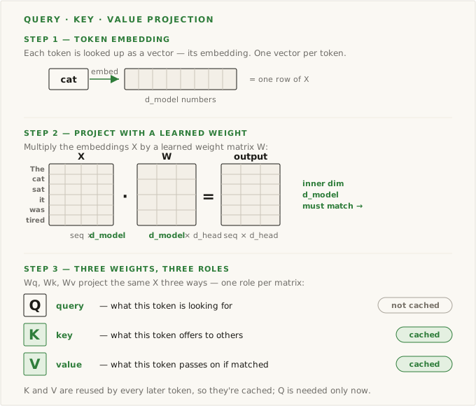
Here’s the move that makes that work. From each token’s embedding, the model produces three vectors, by multiplying it by three learned weight matrices:

• a query ($Q = X W_q$) — what this token is looking for;
• a key ($K = X W_k$) — what this token offers to others;
• a value ($V = X W_v$) — what this token actually hands over if attended to.

The retrieval analogy is exact: a query is a search request, a key is the label on a drawer, a value is what’s inside. Attention matches each token’s query against every token’s key to decide which drawers to open, then pulls out a weighted mix of their values. The three roles are separate on purpose — what a token advertises ($K$), what it searches for ($Q$), and what it contributes ($V$) are different — so the model learns three independent sets of weights.

The shapes matter, because they’re where the cost will come from. If the sequence has $\text{seq}$ tokens and each embedding has width $d_\text{model}$, then $X$ is $\text{seq} \times d_\text{model}$. Each weight matrix is $d_\text{model} \times d_\text{head}$, so each of $Q$, $K$, $V$ comes out $\text{seq} \times d_\text{head}$ — one row per token (Figure 1). Hold onto $K$ and $V$ in particular: those two are exactly what the KV cache stores.

Scaled dot-product attention

The whole operation is one line:

$$\mathrm{Attention}(Q, K, V) = \mathrm{softmax}\!\left(\frac{Q K^\top}{\sqrt{d_\text{head}}}\right) V$$

Score, scale, mask, normalize, blend — five steps, each earning its place. With $Q$, $K$, and $V$ in hand:

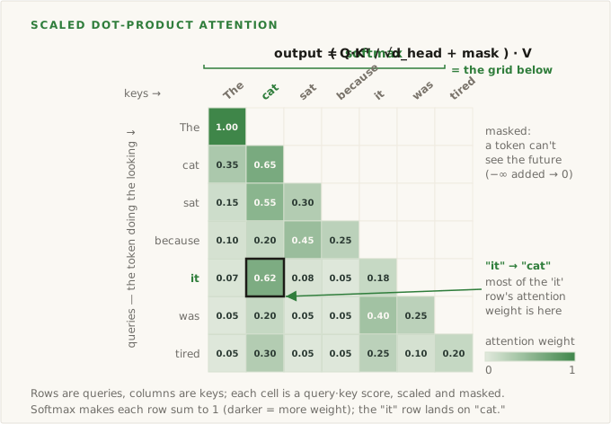
Score every pair. Take the dot product of each token’s query with every token’s key: $\text{scores} = Q K^\top$. A dot product is large when two vectors point the same way and near zero when they’re unrelated, so it’s a natural similarity score: $\text{scores}_{ij}$ is how much token i’s query matches token j’s key — how relevant token j is to token i. The whole point of training $W_q$ and $W_k$ is to learn to aim a token’s query in the same direction as the keys of the tokens it ought to care about. With $\text{seq}$ tokens this is a $\text{seq} \times \text{seq}$ grid, one row per querying token, one column per token being looked at.

Scale it down. Divide every score by $\sqrt{d_\text{head}}$. This looks like a fudge factor and isn’t. A dot product over $d_\text{head}$ dimensions is a sum of $d_\text{head}$ products; the more dimensions, the larger that sum tends to grow, and big raw scores push the next step — softmax — into a corner where one token grabs nearly all the weight and the gradients flatten out. Dividing by $\sqrt{d_\text{head}}$ keeps the scores in a sane range so the model can actually learn which tokens matter.

Mask the future. This is the causal part, and it’s load-bearing for everything downstream. Token it may attend to The cat sat because, but not to was tired — those come after it, and at generation time they don’t exist yet. So before the next step we set every score where $j > i$ to negative infinity, which the softmax will turn into zero weight. The grid becomes lower-triangular: each token sees itself and everything to its left, nothing to its right (Figure 2).

Normalize into weights. Run softmax across each row. Now every row is a set of non-negative weights that sum to one — a probability distribution over “how much of my attention goes to each earlier token.” Why softmax and not just divide each row by its sum? The exponential inside it rewards the largest scores disproportionately, so attention can commit — pour almost all of its weight onto the one or two tokens that matter — while staying smooth and differentiable, a soft version of “pick the best.” Plain normalization would smear the weight too evenly to resolve a sharp reference. In our sentence, the row for it puts most of its weight on cat; that single bright cell is attention doing its one job.

Blend the values. Finally, multiply those weights by $V$: $\text{output} = \mathrm{softmax}(\text{scores} / \sqrt{d_\text{head}})\, V$. Each token’s output is a weighted average of the value vectors of the tokens it attended to. it walks away carrying mostly cat’s value — it has pulled the context it needed. That enriched vector is what attention contributes, and it gets added back into the token’s residual stream — the skip-connection from the last post — so the next layer starts from an it that already knows it’s the cat.

Everything else in this post is consequences.

Many heads

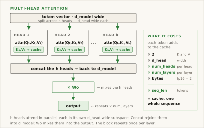
One set of $Q$, $K$, $V$ learns one notion of relevance, but tokens relate in several ways at once (it wants cat; a verb wants its subject). So real transformers run multi-head attention: split the projections into $h$ independent $(Q, K, V)$ triples — each $d_\text{head}$ wide, with its own weights — run the same scaled-dot-product in each in parallel, then concatenate the $h$ outputs and pass them through one final matrix, $W_o$ (Figure 3).

That last matrix isn’t bookkeeping. Concatenation only stacks the heads side by side — they haven’t interacted yet. $W_o$ (shape $d_\text{model} \times d_\text{model}$) is what mixes them: it blends each head’s separate finding into one vector and projects it back into the residual stream, so the next layer sees one combined representation, not $h$ disjoint ones.

The heads share the width rather than each taking the full $d_\text{model}$, so $d_\text{model} = h \times d_\text{head}$. Llama 2 7B splits $d_\text{model} = 4096$ into $h = 32$ heads of $d_\text{head} = 128$ — the same arithmetic, reshuffled into parallel subspaces. So extra heads are nearly free in compute.

The cache is the exception. Every head keeps its own keys and values, so the cache isn’t one $K$/$V$ per token — it’s $\text{num\_heads}$ copies wide (32 for Llama 2 7B). What’s free in arithmetic is paid for in memory; that asymmetry is the hinge between this post and the next.

Where it sits, and what it costs

For one sequence, the KV cache is a product:

$$\text{cache} = \text{num\_layers} \times \text{num\_heads} \times 2 \times \text{seq\_len} \times d_\text{head} \times \text{bytes}$$

Read it as a stack of for every: for every layer, every head stores a key and a value (the $2$), each $d_\text{head}$ wide, for every one of the $\text{seq\_len}$ tokens — times the bytes per number. These keys and values are computed once and kept; recompute them each decode step and generation goes quadratic. And since the causal mask only lets a token look left, earlier entries never change — each step appends one new $K$/$V$ and reads the rest. It’s the $K$ and $V$ of Figure 1, saved once per head, once per layer.

Take Llama 2 7B — 32 layers, 32 heads, $d_\text{head}$ 128, fp16, a 4,096-token context:

$$32 \times 32 \times 2 \times 4{,}096 \times 128 \times 2\ \text{bytes} \approx 2\ \text{GB}$$

That’s 2 GB for a single sequence — not the weights, not the batch, just one conversation’s keys and values. It’s the number behind “the KV cache caps concurrency”: serve a handful at once and the cache, not the math, is what fills the GPU.

And it’s the same row you watched grow in the last post’s KV-cache figure — only now you can see what’s in each entry. Each entry is a key and a value, born from $X W_k$ and $X W_v$, multiplied out by head and by layer. The memory wall wasn’t a property of the serving system. It was sitting in the attention formula the entire time.

What comes next

That’s attention from the bottom up. The $K$ and $V$ it stores for every head, in every layer, are the KV cache. Which raises the obvious question: if the cost is a copy of $K$ and $V$ for every head in every layer, can we keep fewer without losing what attention buys us? That’s the next post — MQA, GQA, MLA, and FlashAttention, which never even writes the $\text{seq} \times \text{seq}$ score grid to memory. Same operation, reshaped to be cheap.